Wave propagation calculation tool (for free-space and 2 wave model)
By inputting parameters for frequency, transmit power and distance, it is possible to calculate the wave propagation characteristics for free-space and 2-wave model.
Basic input parameters
❶ Input the radio frequency in MHz
Frequency MHz
❷ Input the radio transmission power in dBm
Transmission power dBm -->
❸ Input the propagation distance in meters
Distance m
Advanced input parameters
❹ Antenna height
At transmitter m
At receiver m
❺ Antenna gain
At transmitter dBi
At receiver dBi
Log / linear
Explanation of the free-space and 2-wave model
Free-space
Propagation in a perfect vacuum without wave reflection. Theoretically, the received power drops off with the square of the distance.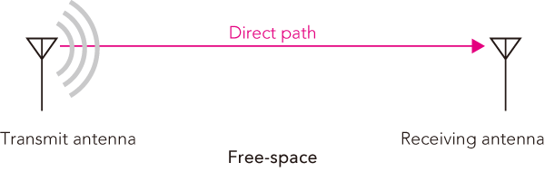
2-wave model
Propagation over an infinitely flat reflective surface. Interference will occur at the receiver when the two waves converge, one having taken a direct route and the other that has been reflected. If they both converge with opposite phase, the overall received power will be less (dead point). The dead points occur more frequently at closer distance to the transmitter. To avoid such areas the receiver will need to be relocated to places where the received power level is at maximum. Using higher frequencies (with shorter wavelengths), the number of dead points will occur more rapidly especially near the transmitter.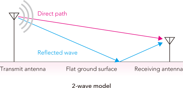
In reality, reflections can occur from buildings and mountains creating multipath propagation (delayed wave arrival) so the situation becomes more complex.
Formulas used on this page
Free space
Propagation loss
The equation describing propagation loss given frequency f (MHz) and distance d(m) from transmitter is:
$$ Loss(dB)=20\log(\frac{4πd}{λ}) $$
where λ is:
$$ λ=\frac{c(^m/_s)}{f(MHz)}=\frac{3\times10^8}{f\times10^6} $$
2-wave model
The tool displays the electric field and received power in free space using the 2 wave model.
Path difference
By using symmetry and applying Pythagoras theorem on the 2-wave model, we can calculate the path difference r(m):
Transmitter antenna height: ht(m)
Receiver antenna height: hr(m)
Distance between the transmitter and receiver antenna: dA(m)
Wave direct path distance: dB(m)
Path difference between direct and reflected wave: r(m)
$$ r(m)=\sqrt{d_A^2+(h_t+h_r)^2}-\sqrt{d_A^2+(h_t-h_r)^2} $$
The electric field strength in V/m (and converted to dBV/m and dBuV/m) at a distance dB(m) from the transmitter outputting pt watts using antenna with gain Gt in dBi is as follows:
$$ E(^{V}/_m)=\biggl(\frac{\sqrt{30p_t10^{(G_t/10)}}}{d_B}\biggr) $$
$$ E(^{dBV}/_m)=20\log\biggl(\frac{\sqrt{30p_t10^{(G_t/10)}}}{d_B}\biggr) $$
$$ E(^{dBuV}/_m)=20\log\biggl(\frac{\sqrt{30p_t10^{(G_t/10)}}}{d_B}\biggr) + 120 $$
Given the wavelength, the phase difference between the 2 waves can be derived from the path difference, r(m). Which can then be used to calculate the combined electric field Er relative to the original electric field E of the direct wave.
We can subtract the loss, Le (dB) due to the environment. So the equation becomes:
$$ E_r(dBV/m)=20\log\biggl[2E\ sin(\frac{\pi r}{\lambda})\biggr]-Le(dB) $$
By converting Er(dBV/m) to absolute value, Er(V/m):
$$ E_r(V/m) =10^{E_r(dBV/m)/_{20}}\ $$
Applying the Poynting vector, to convert electric field to power density, Pu in W/m2, we get:
$$ P_u(W/m^2)=\frac{E^2_r}{120\pi} $$
The receiving antenna aperture (area) is given by:
$$ A_e(m^2)=\frac{\lambda^2}{4\pi}G_r $$
where Gr is the receiver antenna gain (not expressed as dB)
Then total power received by the antenna is therefore:
$$ P_r(dBW)=10\log\biggl\{\biggl(\frac{{E_r^2}}{120\pi}\biggr)\biggl(\frac{\lambda^2G_r}{4\pi}\biggr)\biggr\} - Le(dB) $$