Introduction to the Smith Chart - Part 1
Introduction
The Smith Chart is a useful graphical tool to the RF design engineer who needs to amongst many things, analyse impedances or design matching circuits. Rather than perform many tedious calculations by hand, results can be easily visualised on such a chart, making the RF design engineer's life much easier. Although normally plotted by hand, some RF measuring equipment can take this one step further and display a Smith Chart electronically. Below is an example of a handheld vector network analyser (VNA) with a test load of 50 ohm used for calibration and a screenshot of a Smith Chart from a professional VNA.
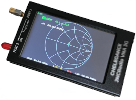
A vector network analyser displaying Smith Chart
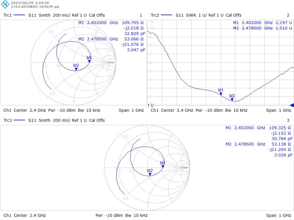
A Smith Chart being shown electronically.
History
The Smith Chart was conceived by Philip Smith, an engineer at Bell Laboratories in the 1930s - in an attempt to avoid the complex calculations associated with RF design and to obtain solutions more quickly. His solution was the Smith Chart which is still widely used today.
Derivation
Before introducing the Smith Chart, first we need to understand circuit impedance.
Impedance
In the previous article, "Impedance and Standing wave ratio", we touched on impedance in relation to antennas. The article explains that impedance Z contains reactance X and resistance R denoted by the following formula:
$$Z = R + jX$$
The impedance, resistance and reactance unit is in ohms (Ω) and the reactance jX, with the complex operator, indicates the reactance has an orthogonal relationship to the resistance value as you will see later. If reactance X was zero (for example in a simple resistor), the impedance will be a pure resistance.
Real antennas contain both resistance (often referred to as radiation resistance) and some reactance. For antennas, reactance is generally undesirable as it does not contribute any energy to the emitted radiation.
Calculating magnitude of reactance
The values for reactance depend on signal frequency in Hertz (Hz) and the inductor/capacitor values, L and C in Henries and Farads respectively.
Inductor reactance written as XL
$$X_{L} = 2\pi f L$$
Capacitor reactance written as XC
$$X_{C} = \frac{1}{2\pi f C}$$
The unit of reactance is in ohms (Ω) and here only their magnitudes are shown. We will see shortly that reactance can be negative or positive when expressed using the j operator.
The complex plane
By knowing resistance R and reactance X, these will map a point on a 2 dimensional plane (known as a complex plane). The "j" indicates the reactance has an orthogonal relationship to the resistance and can be positive or negative, meaning that the magnitude of the impedance Z will be a line drawn out from the centre to the plotted value. We can do this for 3 example circuits shown below.
Representing impedances on a complex plane. ZA, ZB, ZC, XL and XC are in ohms.
From the graph, we can note that:
- If the circuit has pure resistance (zero reactance), Z will lie on the horizontal axis.
- Inductors L introduce positive reactance and shifts Z upwards.
- Capacitors C introduce negative reactance and shifts Z downwards.
Adding resistances and reactances in series
If resistors, inductors and capacitors are in series, the resistances R and reactances X can be added:
Adding reactance in series. ZTotal , R and X are in ohms. The circuit contains mostly inductive reactance.
The Smith Chart
Turning the complex plane into a Smith Chart
To someone unfamiliar with the Smith Chart, it can appear unusual and complex. However, its origin is straight forward to explain as we shall see.
Look at the previous chart and imagine holding the ends of the reactance axis and bending them into a circle so they intersect with the resistance axis as shown:
Transformation of the complex plane into the Smith Chart
Then the vertical resistance lines become circles of constant resistance and the horizontal reactance lines become lines of constant reactance. In other words, all points on a resistance circle have the same resistance and all points on a reactance line have the same reactance. The intersection of the circles and lines represent the impedance and can be read off the chart.
Normalisation
In practice, an RF engineer may encounter very small or very large values of resistances and reactances. To include all of them on the same chart would be impractical.
To solve this, engineers use a process called "normalisation" when plotting values on the chart. A reference value (usually the characteristic impedance, Zo of the system) is chosen and our resistance and reactance values are divided by this reference value to obtain the normalised impedance Z'. If we assume that Zo is 50 ohms for RF communication, then:
$$Z' = \frac{R+jX}{50} = \frac{R}{50}+j\frac{X}{50}$$
If the normalised scale is used on the Smith Chart, the centre point will have a value of 1 (in this case, 50 ohms) with the end points representing short and open circuit.
Example impedance plots
We can plot some example impedances below. For simplicity we represent our components using their resistance and reactance values, as the Smith Chart cannot operate on component values directly. This is not a problem as conversion to component values can be done at a later stage.
Both the actual impedance Z and normalised impedance Z' are shown below:
Example plots with components shown by their resistances and reactances only. ZA ,ZB and ZC are in ohms
The engineer can manipulate the impedance to any position in the chart by the addition or removal of components. The goal is that every adjustment will move the point until it reaches the desired position in the Smith Chart. In the following example, we will look at a simple impedance transformation using the Smith Chart.
Impedance matching example
Consider a load ZLoad that has impedance in ohms and that this load is connected to a signal generator of 400 MHz. For example:
$$Z_{Load} = 50 - j40$$
The resistance part is 50 ohms, but also includes some reactance of -j40 ohms. Let us assume that we would like to present to the generator, a purely resistive 50 ohm load (shown by Zin). Then we need to insert a matching network between the generator and the load.
Matching impedance example (generator not shown)
As the load reactance is negative, this implies it has some capacitance that we will need to cancel out with an inductor inserted in series. How can we use the Smith Chart to get the value of inductor needed?
First we need to normalise ZLoad so we can plot it on our chart. Note that the apostrophe (') denotes the normalised value.
$$Z_{Load}' = \frac{50}{50}-j\frac{40}{50} = 1 - j0.8$$
Due to the capacitance, the point lies below the resistance axis. For matching, the point should be moved to the centre which would transform it to a load containing purely 50 ohms resistance. To move the point to the centre, we imagine applying an equal amount of positive reactance (jX'L = +j0.8), implying the use of an inductor.
Applying a positive reactance for our matching section
So we can un-normalise the X'L = 0.8 to get the reactance value for our inductor.
$$X_{L} = X_{L}' \times 50 = 0.8\times50$$
$$X_{L} = 40 Ω$$
Transforming this to the inductor value in H, using the formula near the top of this page.
$$L = \frac{X_{L}}{2 \pi f}$$
$$L = \frac{40}{2 \pi \times 400,000,000}$$
$$L \approx 16 \times 10^{-9}$$
$$L \approx 16nH$$
Building our matching network
Note that the calculation could be done without the Smith Chart, as we would deduce that the inductor reactance needed would be equal to the capacitor reactance we are trying to cancel out. However for more complex circuits, calculations would become more tedious and it would be better to use the Smith Chart.
Conclusion
We now conclude part one of this article.
So far we have focused on the impedance Smith Chart (the standard Smith Chart) and performed a simple transformation example. However in the second part, we will introduce another Smith Chart known as the admittance Smith Chart that covers components in parallel. When combined with the standard Smith Chart, any circuit containing series and parallel components can be analysed making the Smith Chart an even more powerful tool.