Propagation
How radio waves propagate?
In the article, How antennas radiate?, we established that radio waves are produced from an energy source consisting of oscillating magnetic and electric fields. These radio waves radiate outwards at the speed of light (300,000,000 m/s in a vacuum). Their motion resembles the movement of ripples in a pond.
Many people assume that radio waves travel a fixed distance after which they are no longer receivable. While its true that the radio waves do become weaker the further out they travel, as long as they are still distinguishable from the noise, they can still be received. For example, the Voyager spacecraft launched in 1977 are now many billions of kilometres away but thanks to the Deep Space Network, communication is possible with extremely large parabolic "dish" antennas with very high gain.
Predicting how the radio wave travels can be difficult as the environment has a large influence. So to assist the engineer during the design of the radio system, this article introduces Circuit Design's various calculation tools for radio wave propagation.
Factors that limit radio wave propagation
Radiated power
Increasing the radiated power will improve the chances of signal reception at the receiver. Even so, it may introduce other problems such as radio signals ending up where they are not suppose to and causing interference to other users. Radio regulations cover many parameters, one of which is EIRP which limits radiated power. (refer to Gain (EIRP and ERP) for more information)
Also higher transmit power generally means higher current consumption which maybe a problem if batteries are used.
Frequencies used
Generally speaking lower frequency waves travel further than higher frequency waves. For example, people ask why AM radio waves can be heard from many hundreds of kilometres away, but why FM radio waves are only heard locally and assume there is something characteristic about AM. But the actual reason is that AM historically used lower frequencies (in the LF* to HF* frequency range) and there are certain propagation mechanisms (such as atmospheric skip) that enable low frequencies to travel around the globe.
So higher frequencies such as 2.4 GHz travel e.g. few hundred metres compared to several hundred metres at 434 MHz.
* LF: Low Frequency, HF: High Frequency
Antenna positioning
Buildings and trees can block the signal so if possible the antennas should be placed high up to clear them. In addition antennas must maintain a zone of clearance between them called the Fresnel Zone (described later in this article). The Fresnel clearance becomes smaller at higher frequencies so it will be antenna placement and not necessarily height that optimises communication.
Noise and interference susceptibility
In the environment, there exists many sources of electrical noise (e.g. lights, ignition systems, motors). AM and ASK signals are the most susceptible since noise only adds to the amplitude variations. On the other hand, FM and FSK signals are more robust as the received signal only depends on frequency variations.
In digital communications with many users sharing the same frequency band, various encoding schemes such as frequency hopping and direct sequence spread spectrum allow reliable communication where interference is high.
Obstructions
The places with few or no obstructions where communication can happen effectively include open waters, ground to aircraft and satellite communications. In most cases however, communication takes place in and around buildings, around trees and mountains etc. There are several ways radio waves can interact with objects as shown.
Various propagation paths
Absorption and reflection
When a radio wave strikes a flat surface, some waves will be reflected, absorbed or pass through the material. The amount of each depends on the obstruction composition. A perfect conductor (e.g. metal, sea water) reflects all radio waves.
Some materials are able to absorb almost all radio waves. An example material found in anechoic chambers uses RF absorbing foam impregnated with a metallic material such as carbon, iron and ferrite.
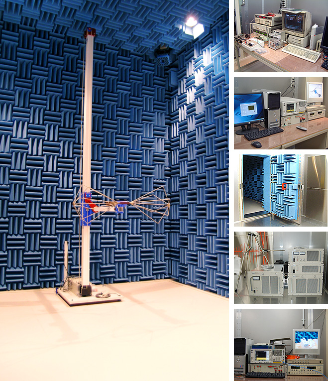
Radio wave absorbing material used on walls and ceiling of the anechoic chamber
Diffraction
According to Huygen's principle, every point on a wave front acts as source of secondary wavelets which combine to produce a new wave front in the direction of propagation. When these wavelets are allowed to enter the shadowed region created by the obstruction, the result is diffraction which allows the radio wave to "curve" around obstacles. The amount of this "curving" behaviour depends on the wavelength. Lower frequencies such as the AM broadcast band can travel around mountains easily (due to the larger wavelengths) allowing waves to travel over the ground for long distances (called ground waves).
Higher frequencies with their shorter wavelengths are much less diffracted relying more on line of sight.
Communication medium
Generally speaking the more dense the material, the more trouble radio waves will have propagating through the material. You will have noticed this when the radio or your GPS stops working when entering a tunnel. Even if the surrounding soil is not so dense, the large amount is enough to block the radio waves. Very dense materials such as lead or concrete used for x-ray and gamma shielding will also block radio waves.
Regarding liquids, it is possible for radio waves to travel but seawater is a problem as it is conductive. In these conditions, MHz frequencies cannot be used so submarines use 3 - 30 kHz (Very Low Frequency) for communication.
Fading
Due to the various propagation paths mentioned, the receiver sees radio waves that are phase shifted from each other. As these waves combine, the receiver encounters both high and low level reception spots. This is known as fading.
Doppler effect
In mobile communications, if the transmitter and receiver are moving away from or approaching each other, the result is a small frequency drift from the carrier frequency. This is similar to what occurs with sound waves, where the sound from a passing ambulance with a siren will seem to change in pitch. The severity of the frequency drift depends on the wavelength and relative speed between the transmitter and receiver. In everyday situations, the speed of the radio wave is very high and any drift would be imperceptible. Any fluctuations in signal level would instead likely come from e.g. signal reflection.
Propagation models
We established that radio waves have various modes of propagation. To realise this mathematically, there are standard models that can be used as a basis when designing your radio system.
Free space model
The simplest model is propagation in free space.
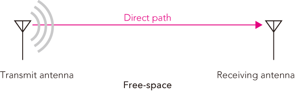
The level seen at the receiver decays as a function of transmitter-receiver separation distance d (metres) and also wavelength λ (metres). Mathematically, it can expressed as:
$$ \text{Path Loss(dB)} = 20\log(\frac{4πd}{λ}) $$
As this is a power law function, if I double my distance, the power at my receiver is only a quarter of the power at the transmitter.
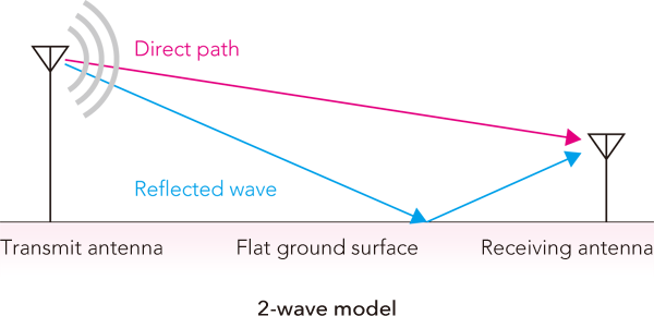
The 2 path model
If a reflective surface exists, the radio wave will follow 2 paths - a direct path and a reflected path. There will be a length difference between both paths with the receiver seeing another identical wave, but delayed. This delayed signal can add to or subtract from the direct signal depending on the phase difference.
If we assume constant frequency, this phase difference depends on the path difference which in turn depends on the antenna height and separation between the transmitter and receiver. If we take an example where the transmitter is a base station and the receiver is a mobile station - then if we move further from the base station, we can expect the interference between the 2 waves to produce a larger signal or a smaller signal.
Wave propagation calculation tool example
Circuit Design has a calculation tool to demonstrate the difference between free space and the 2 path model. In practical communications, there are other losses in addition to the free space loss. If obstructions are not too severe, one can normally use the 2-path model as an approximation.
Let us use an example signal at 434 MHz, 10mW RF power using 2.14 dBi antenna for transmitter and receiver. Let the antenna height be 5m and the distance between them be 200m. For the 2 path model, the propagation behaviour is erratic with interference between the 2 waves causing many signal drop offs especially at close range. Susceptibility to drop offs are dependent on wavelength, meaning that at higher frequencies, drop offs become much more frequent.
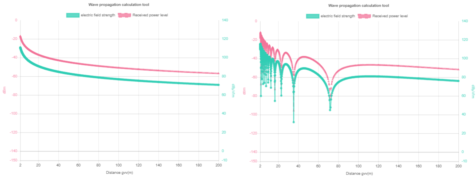
Free space (left) and 2 path model (right)
Fresnel zone
Line of sight communication does not only mean seeing each other's antennas but also requires certain amount of clearance from objects. This zone of clearance is called the Fresnel zone and must be maintained to avoid any signal loss.
When radio waves radiate, every point on the wave produces secondary wave fronts. This means that the receiver does not see all the radio wave travelling in a single plane, but also slightly above and below it with the direct path contributing the most energy. Any obstruction that blocks these wave fronts will attenuate the signal. Therefore it is important to keep this area clear of any obstructions.
1st Fresnel zone - obstructed and clearing the obstruction by raising antenna height
Fresnel zone calculation tool
Circuit Design includes a calculation tool which calculates the minimum antenna height off the ground in order that the Fresnel zone is not obstructed. If the antennas are placed that ensures at least 60% of the Fresnel radius is cleared, signal level will not be significantly affected.
Note that the Fresnel zone becomes smaller with higher frequency/shorter transmitter and receiver distance. If it is difficult to get line of sight then the antennas need to be installed in the most optimum location. Regarding the installation height of the antenna, it maybe necessary to consider other factors such as height pattern as well as the Fresnel zone.
Antenna height pattern
Once the antenna location is decided, the exact height of the receiving antenna needs to be adjusted in order that the signals arrive at the antenna in phase. This can be achieved by moving the antenna up and down while monitoring the received signal level. To assist the engineer, Circuit Design provides a calculation tool that gives the height pattern pitch in metres. You should be able to find the signal peak in this range.
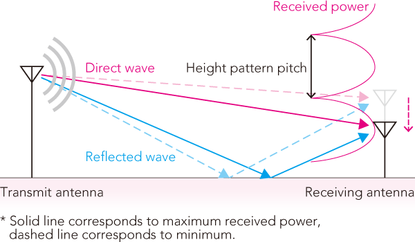
Height pattern pitch
Okumura Hata model
The Okumura Hata model is a model for predicting mature cellular and land mobile communication systems in various environments involving open land, suburbs, medium cities and large cities. Designed for distances involving 1 to 20km, distances below this range - the values are not as reliable. Also the actual environment can differ to what was used to take the measurements so this tool should be used as a basic predictor for reception. The conditions applied to this model and the following calculation tool are as follows:
Frequency f(MHz):150 MHz to 1.5 GHz
Communication distance d(m):1 km to 20 km
Base station antenna height hb(m):30 m to 200 m
Mobile antenna height hm(m):1 m to 10 m
Okumura-Hata curve calculation tool
To use the calculation tool, click here to visit the page.
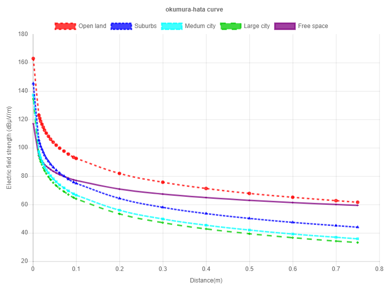
Okumura Hata curves calculated based on the parameters entered
Input the frequency in MHz, the transmitter output power, antenna height, gain and distance. The graph will show either electric field strength up to the distance specified or the corresponding output power from the receiver antenna.
Conclusion
The topic of propagation is extremely large with much of it beyond the scope of this article. This article is meant as a guide for the engineer when designing his/her radio system without touching too much on the mathematical concepts. However for reference purposes, the formulas used for calculation are included in the calculation tool pages.