Confirming radio conditions in advance
Introduction
Unlike wired systems, wireless systems are dependent on the frequency band used, distance, radio equipment installation and any obstacles in the environment, as well as emissions from other radio systems and equipment. So Circuit Design recommends you thoroughly check the radio propagation conditions before installing any wireless system.
This article mentions detailed methods for confirming propagation conditions. They can be broadly divided into 2 areas - simulation and equipment testing.
Simulation
Simulation can be used mainly to check the propagation conditions before confirmation with the actual radio. Even without using the actual radio, it is possible to check the propagation conditions to some extent by entering the radio specifications, details of the location and other conditions.
Circuit Design simulation tools
On the Circuit Design website, there is a calculation tool that allows you to simulate the received signal level.
Wave propagation calculation tool (for free-space and 2 wave model)
If there are only relatively few obstructions, the received level can be simulated by selecting the 2-wave model.
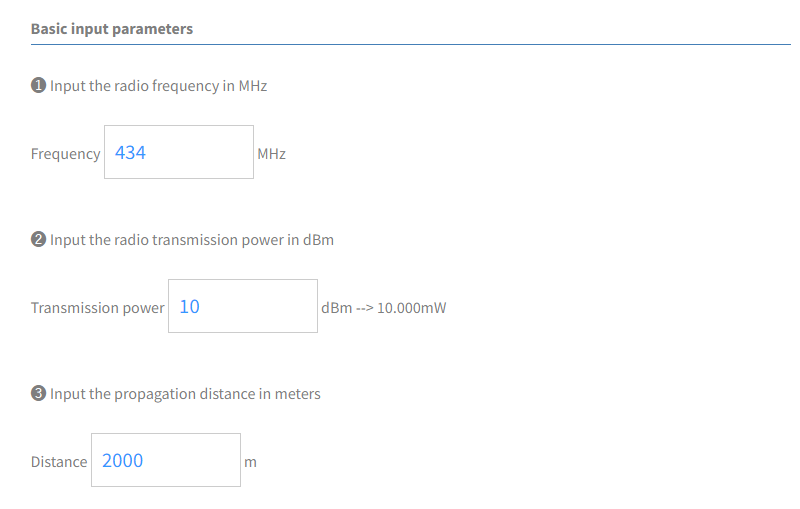
We can input basic and detailed parameters according to the conditions below. Here we use an example of low power radio module at 434 MHz.
The basic parameters to be input are frequency of use, transmitter power and communication distance.
Detailed parameters to be entered are height of transmit/receive antenna as well as their gain. Again we are using the 2-wave model.
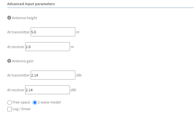
By inputting the above parameters, we can determine the calculated received signal level.
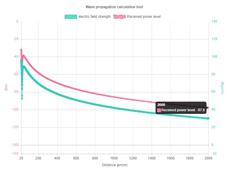
We can see from the graph that radio waves get weaker with distance (but does not go down to zero). In this case, we can see the received signal level of -97.8 dBm at a distance 2000 m away. So can communication be achieved at this distance? It depends. We need to consider is this level just enough for the receiver to demodulate the signal allowing a range of acceptable bit error? This level referred to as receiver sensitivity is different for all radio receivers, so for example where the radio receiving sensitivity was -110 dBm (Bit error rate 1%), a margin of 10 dB may not be sufficient for stable communication. However communication would still be possible to some extent depending on the application requirements.
Wave propagation calculation tool (for free-space and 2 wave model)
Okumura-Hata curve calculation tool
In a similar manner, one can input basic and detailed parameters and perform a similar simulation.
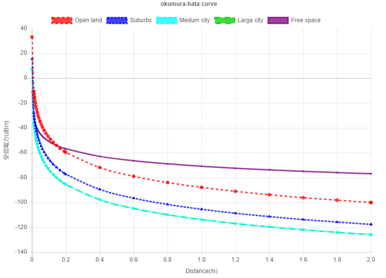
The Okumura-Hata curve can perform simulations in 5 different environments - open land, suburbs, small-medium cities, large cities and free space.
These approximation curves were originally aimed for medium to long distance, i.e. several km to 20 km using frequencies 150 to 1500 MHz. Beyond these values, the discrepancy between the actual and simulated results will be higher.
Okumura-Hata curve calculation tool
Terrain simulation
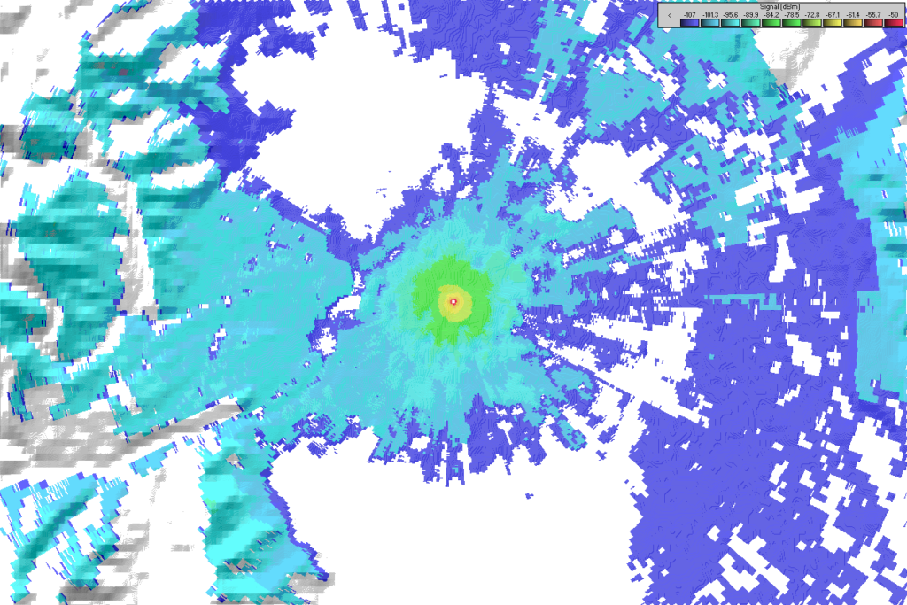
Simulation can be performed based on terrain information. Such tools are available on the internet and when used can output results matching the characteristics of the terrain.
As with the Circuit Design calculation tools, you can see the possible communication area by setting the threshold level that takes into account the receive sensitivity level and margin.
For example, the tool, "Radio Mobile" developed by Canadian amateur radio enthusiast (VE2DBE) was used to perform simulation around the Circuit Design premises. By using the output data, it was possible to produce a plot with tools such as google maps.
Confirmation with actual equipment
From the above simulations, you can somewhat judge if communication is possible. However without performing communication in the actual location, it is not possible to know for certain. For example its worth stating that if there is a high level of noise or the desired frequency is already in use by another system, communication may not be possible. As the simulation results are only a guide, it is necessary to confirm using actual equipment before introducing a wireless system in that location.
In this article, we will show some confirmation examples using Circuit Design MU series of modems and the evaluation software.
Received signal strength (RSSI) confirmation
Communication can be confirmed using received signal strength for radio modules with RSSI function (ability to show received signal strength).
Noise level and other equipment in use
It is important to assess the suitability of use at the location and the selection of the actual frequency channel by looking at the noise floor. The best way is to measure using a spectrum analyser and other similar equipment. However such equipment can be expensive and requires a certain amount of RF knowledge to use. When using the air monitor featured in the evaluation program for the MU series modem, the resolution and sampling rate will be inferior compared to dedicated measuring equipment; but such measurements can be performed much more easily.
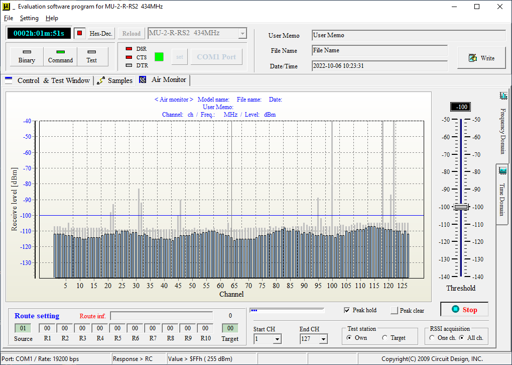
Frequency domain measurement
By looking at the frequency domain, you can check (at a glance), the condition of the chosen frequency channel in the band. It is not enough to check only once and it becomes necessary for example to use the peak hold function to continuously check over a long period of time. By changing sweep time, you can make a number of confirmations. The below graph shows the air monitor after running continuously for 2 hours using the peak hold function. You can see that signals have appeared on channels such as ch100, 118 and 122 along with subtle variations in noise level that would not have been possible to capture with just a few sweeps. By knowing this information, it is possible to avoid using these channels during actual operation. The noise level can fluctuate by several dB over time, so consider that it can vary up to 10 dB if such an observation becomes difficult to confirm.
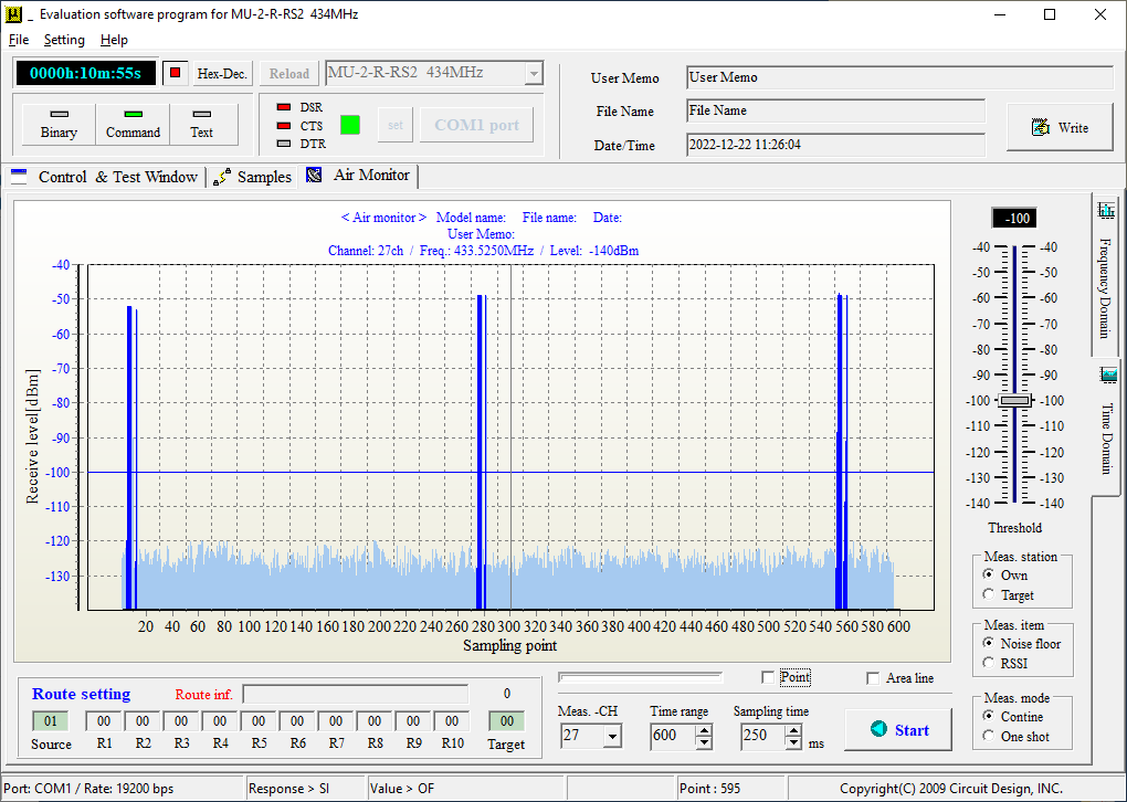
Time domain measurement
The time domain allows you to continuously monitor the received signal strength of a single frequency channel. For example, assume an indication on the frequency domain showing a channel in use (e.g. ch 27). We can view this channel in the time domain and see how it is actually used. For a long sampling time (interval) and using many sample points as shown in the below image, we can verify if a transmission is repeating or whether it is a once only transmission. If the sampling time is too large, detailed events will not be captured and this setting must be adjusted appropriately. The below graph shows a trace on ch 27 indicating a signal occurring once about every minute.
If instead we reduce the sampling time, we can examine a single transmission in much more detail. In the below image, we can see that it contains one peak lasting about 1 second and another lasting just under 0.5s.
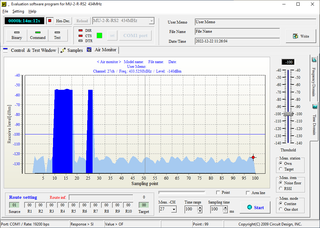
Compared to using actual measuring equipment, some data maybe lost and functions maybe inferior. By devising the best sampling times and range, it is still possible to confirm the signal in detail.
Packet signal level
Even though it is possible to check the received signal level at the target using time domain, the MU series of modems have a command, "@CR" to measure the RSSI of the target station. We describe how the evaluation program can be used to as a way of checking RSSI of the target station through command. By either issuing "@CR" from the local station or clicking "Target: RSSI", it is possible to obtain the value. The response "*DR=04xxXX" is returned. Following the "04", the "xx" represents the received level at the target station during reception (HEX format) and the "XX" represents the noise floor level (HEX format). The minus notation is omitted from the returned values. In the evaluation program, if the "Target: RSSI" is clicked, the level is displayed as text. From this you can judge if communication will be sufficient in your chosen environment.
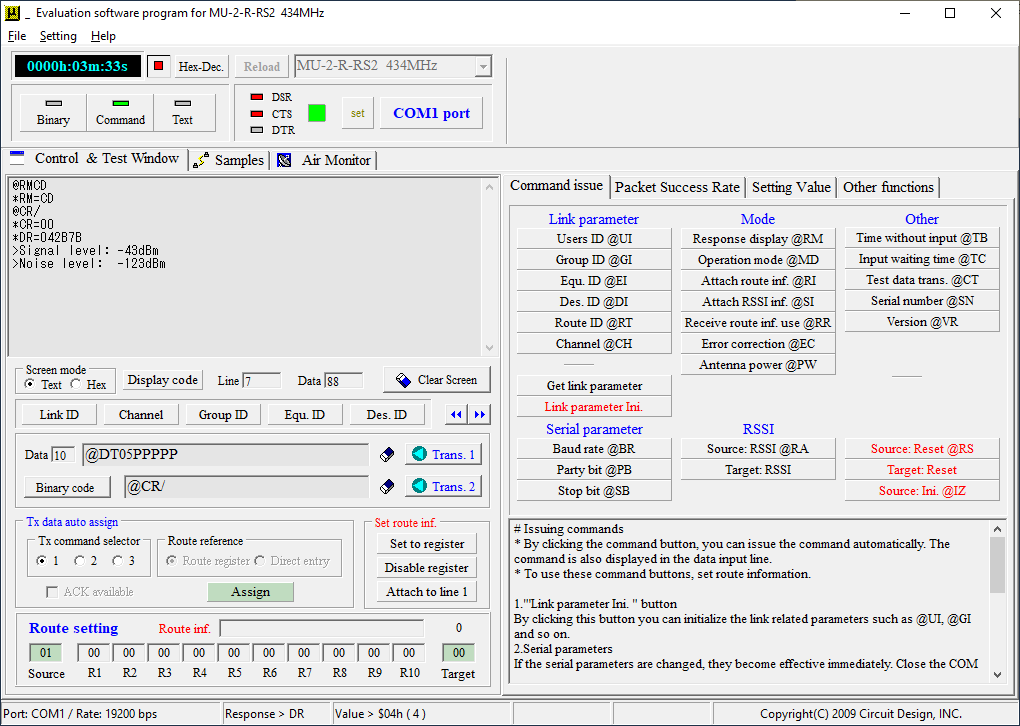
Received level of -43 dBm (0x2B) and noise floor level of -123 dBm (0x7B)
Communication test with actual unit (Packet communication test)
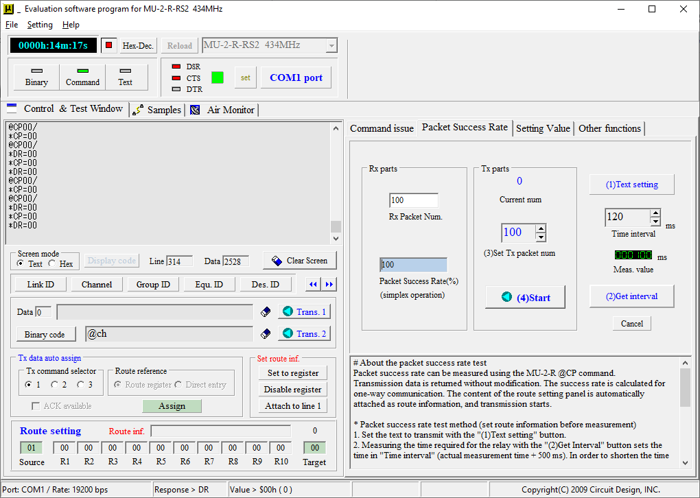
In practice, the communication is performed multiple times between units with the number of transmissions and the returned packets counted. For example, transmitting a packet 100 times with the return of 99 packets would be expressed as a 99% return rate - an approximation of the real radio operation. As with the RSSI, you can get a more precise evaluation by using this over a longer period of time or increasing number of transmissions. This tool is a feature included in the evaluation software. Note that the test describes 2 way communication - for example it is necessary to take into account that an outgoing packet is received correctly but the returning packet is not received correctly leading to the conclusion that communication is unsatisfactory.
Combining RSSI and packet
There are places where either just confirming the signal level or performing packet tests is not enough to fully grasp the communication condition. For example, even just by seeing a high level when looking at signal level alone does not reveal factors such as multipath that can degrade communication performance. Also a packet return rate of 100% when doing packet testing alone means that one cannot visualise the amount of receive margin.
Due to the above, it is recommended that both signal level and packet testing be performed together when using actual radio units.
In the case of checking communication while moving, incorporating the location information to the above can allow you to overlay the results onto a map.
As an example, the location information and signal level while checking around the company premises is plotted in the google map shown below.